Modeling a single voxel

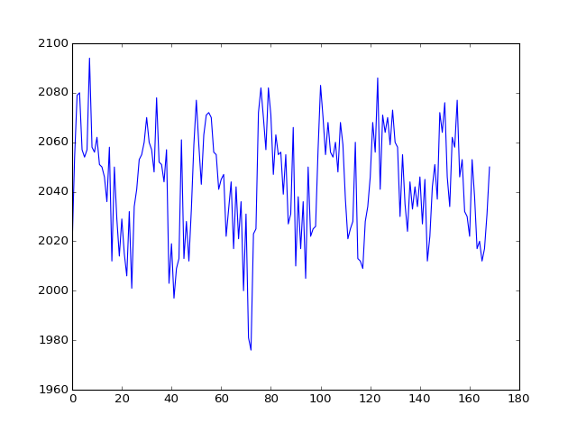
A long time ago (Voxel time courses), we were looking at a single voxel time course.

Let’s get that same voxel time course back again:

>>> import numpy as np
>>> import matplotlib.pyplot as plt
>>> import nibabel as nib

>>> img = nib.load('ds114_sub009_t2r1.nii')
>>> data = img.get_data()
>>> data = data[..., 4:]

The voxel coordinate (3D coordinate) that we were looking at before was at (42, 32, 19):

>>> voxel_time_course = data[42, 32, 19]
>>> plt.plot(voxel_time_course)
[...]

(png, hires.png, pdf)

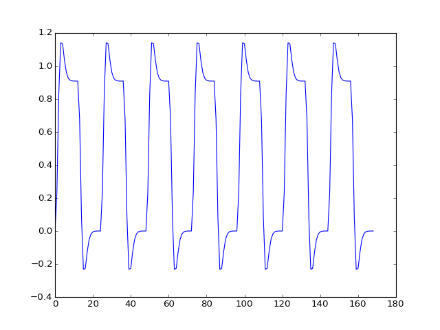
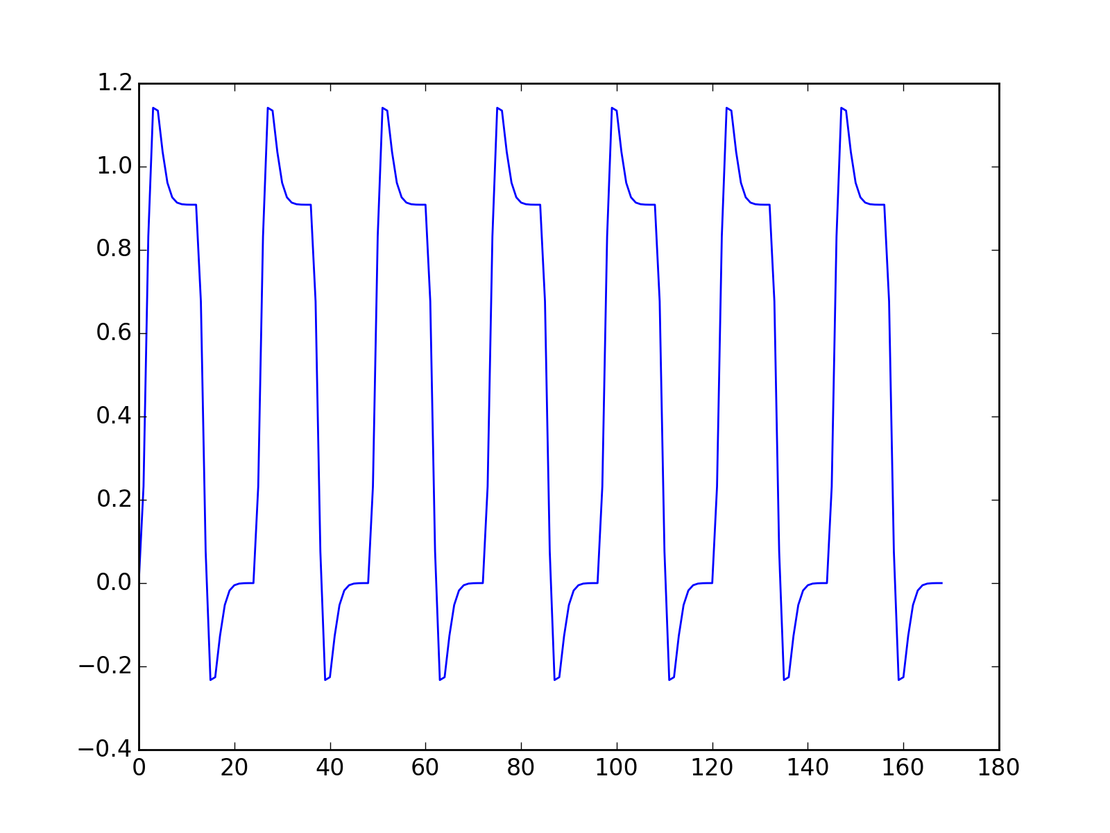
Now we are going to use our new convolved regressor to do a simple regression on this voxel time course.

If you don’t have it already, you will need to download ds114_sub009_t2r1_conv.txt.

>>> convolved = np.loadtxt('ds114_sub009_t2r1_conv.txt')
>>> # Knock off first 4 elements to match data
>>> convolved = convolved[4:]
>>> plt.plot(convolved)
[...]

(png, hires.png, pdf)

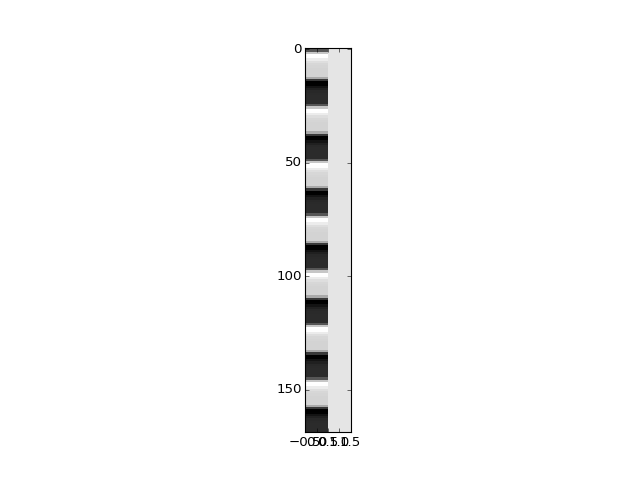
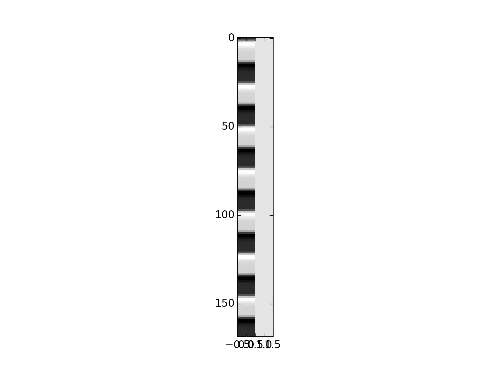
First we make our design matrix. It has a column for the convolved regressor, and a column of ones:

>>> N = len(convolved)
>>> X = np.ones((N, 2))
>>> X[:, 0] = convolved
>>> plt.imshow(X, interpolation='nearest', cmap='gray', aspect=0.1)
<...>

(png, hires.png, pdf)

\(\newcommand{\yvec}{\vec{y}}\) \(\newcommand{\xvec}{\vec{x}}\) \(\newcommand{\evec}{\vec{\varepsilon}}\) \(\newcommand{Xmat}{\boldsymbol X} \newcommand{\bvec}{\vec{\beta}}\) \(\newcommand{\bhat}{\hat{\bvec}} \newcommand{\yhat}{\hat{\yvec}}\)

As you will remember from Introduction to the general linear model, our model is:

\[\yvec = \Xmat \bvec + \evec\]

We can get our least squares parameter estimates for \(\bvec\) with:

\[\bhat = \Xmat^+y\]

where \(\Xmat^+\) is the pseudoinverse of \(\Xmat\). When \(\Xmat\) is invertible, the pseudoinverse is given by:

\[\Xmat^+ = (\Xmat^T \Xmat)^{-1} \Xmat^T\]

Let’s calculate the pseudoinverse for our design:

>>> import numpy.linalg as npl
>>> Xp = npl.pinv(X)
>>> Xp.shape
(2, 169)

We calculate \(\bhat\):

>>> beta_hat = Xp.dot(voxel_time_course)
>>> beta_hat
array([   31.185514,  2029.367685])

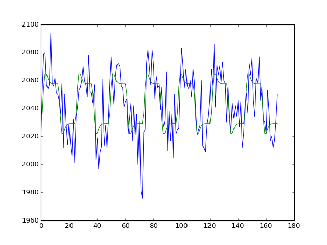
We can then calculate \(\yhat\) (also called the fitted data):

>>> y_hat = X.dot(beta_hat)
>>> e_vec = voxel_time_course - y_hat
>>> print(np.sum(e_vec ** 2))
41405.5727762
>>> plt.plot(voxel_time_course)
[...]
>>> plt.plot(y_hat)
[...]

(png, hires.png, pdf)