Using onsets that do not start on a TR

You’ll need the file new_cond.txt to type along with this demonstration.

>>> from __future__ import division
>>> import numpy as np
>>> import matplotlib.pyplot as plt
>>> import nibabel as nib

Imagine we are analyzing our example image. It has a TR of 2.5, and 173 TRs.

>>> TR = 2.5
>>> n_trs = 173

The actual condition file for this dataset is ds114_sub009_t2r1_cond.txt. You may remember it has a block design with blocks of length 12 TRs while the subject is doing the task.

What if we had a different event related condition file like this:

>>> cond_data = np.loadtxt('new_cond.txt')
>>> cond_data
array([[   3.35,    3.  ,    2.  ],
       [  12.76,    3.  ,    2.  ],
       [  43.27,    3.  ,    2.  ],
       [  75.25,    3.  ,    1.  ],
       [  95.48,    3.  ,    2.  ],
       [ 167.84,    3.  ,    2.  ],
       [ 282.36,    3.  ,    2.  ],
       [ 304.76,    3.  ,    2.  ],
       [ 356.32,    3.  ,    2.  ],
       [ 372.22,    3.  ,    3.  ]])
>>> onsets_seconds = cond_data[:, 0]
>>> durations_seconds = cond_data[:, 1]
>>> amplitudes = cond_data[:, 2]

Notice that the onsets of the events can happen in the middle of the volumes (well after the volumes have started).

>>> onsets_in_scans = onsets_seconds / TR
>>> onsets_in_scans
array([   1.34 ,    5.104,   17.308,   30.1  ,   38.192,   67.136,
        112.944,  121.904,  142.528,  148.888])

Notice also that the events have amplitudes between 1 and 3. The events of amplitude 3 we expect to have an evoked brain response three times higher than events with amplitude 1.

What to do about the events with onsets that don’t exactly align with the start of the TRs (volumes)?

One option would be to round the event onsets to the nearest TR. This will mean that the event model will be different from our expected response by TR seconds / 2 == 1.25 seconds in this case.

Can we do better than that?

One option is to make a neural and hemodynamic regressor at a finer time resolution than the TRs, and later sample this regressor at the TR onset times.

This is what we do next.

>>> tr_divs = 100.0  # finer resolution has 100 steps per TR

With each TR divided into 100 intervals, one element corresponds to time intervals of 1/100 of a TR:

>>> high_res_times = np.arange(0, n_trs, 1 / tr_divs) * TR

We will soon create a new neural prediction time-course where one element corresponds to 1 / 100 of a TR:

>>> high_res_neural = np.zeros(high_res_times.shape)

We have the onset indices in terms of TRs, but now we want the onset indices in terms of the new vector with 100 elements per TR:

>>> high_res_onset_indices = onsets_in_scans * tr_divs
>>> high_res_onset_indices
array([   134. ,    510.4,   1730.8,   3010. ,   3819.2,   6713.6,
        11294.4,  12190.4,  14252.8,  14888.8])

In the same way, the durations were in seconds. We divide by the TR to get duration in terms of scans, then multiply by 100 to get the number in terms of elements in the new high_res_neural time-course.

>>> high_res_durations = durations_seconds / TR * tr_divs
>>> high_res_durations
array([ 120.,  120.,  120.,  120.,  120.,  120.,  120.,  120.,  120.,  120.])

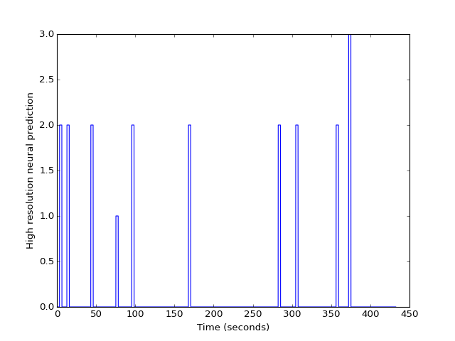
Now we fill in the high_res_neural time course by setting values between the start and the end of each event with the matching amplitudes:

>>> for hr_onset, hr_duration, amplitude in zip(
...            high_res_onset_indices, high_res_durations, amplitudes):
...     hr_onset = int(round(hr_onset))  # index - must be int
...     hr_duration = int(round(hr_duration))  # makes index - must be int
...     high_res_neural[hr_onset:hr_onset + hr_duration] = amplitude
>>> plt.plot(high_res_times, high_res_neural)
[...]
>>> plt.xlabel('Time (seconds)')
<...>
>>> plt.ylabel('High resolution neural prediction')
<...>

(png, hires.png, pdf)

We can use the hemodynamic response function we created earlier:

>>> from scipy.stats import gamma
>>>
>>> def hrf(times):
...     """ Return values for HRF at given times """
...     # Gamma pdf for the peak
...     peak_values = gamma.pdf(times, 6)
...     # Gamma pdf for the undershoot
...     undershoot_values = gamma.pdf(times, 12)
...     # Combine them
...     values = peak_values - 0.35 * undershoot_values
...     # Scale max to 0.6
...     return values / np.max(values) * 0.6

We are going to convolve at this higher time resolution. First we need to sample the HRF at this finer time resolution, to match the neural prediction:

>>> hrf_times = np.arange(0, 24, 1 / tr_divs)
>>> hrf_at_hr = hrf(hrf_times)

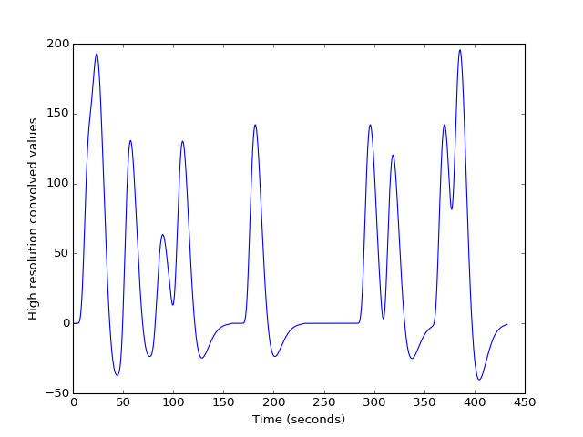
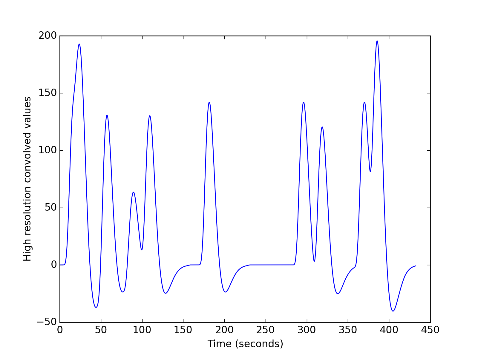
Next we convolve the sampled HRF with the high resolution neural time course:

>>> high_res_hemo = np.convolve(high_res_neural, hrf_at_hr)[:len(high_res_neural)]
>>> plt.plot(high_res_times, high_res_hemo)
[...]
>>> plt.xlabel('Time (seconds)')
<...>
>>> plt.ylabel('High resolution convolved values')
<...>
>>> len(high_res_times)
17300

(png, hires.png, pdf)

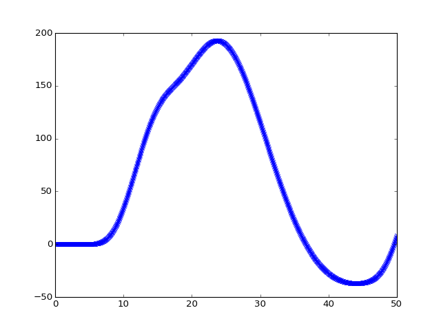
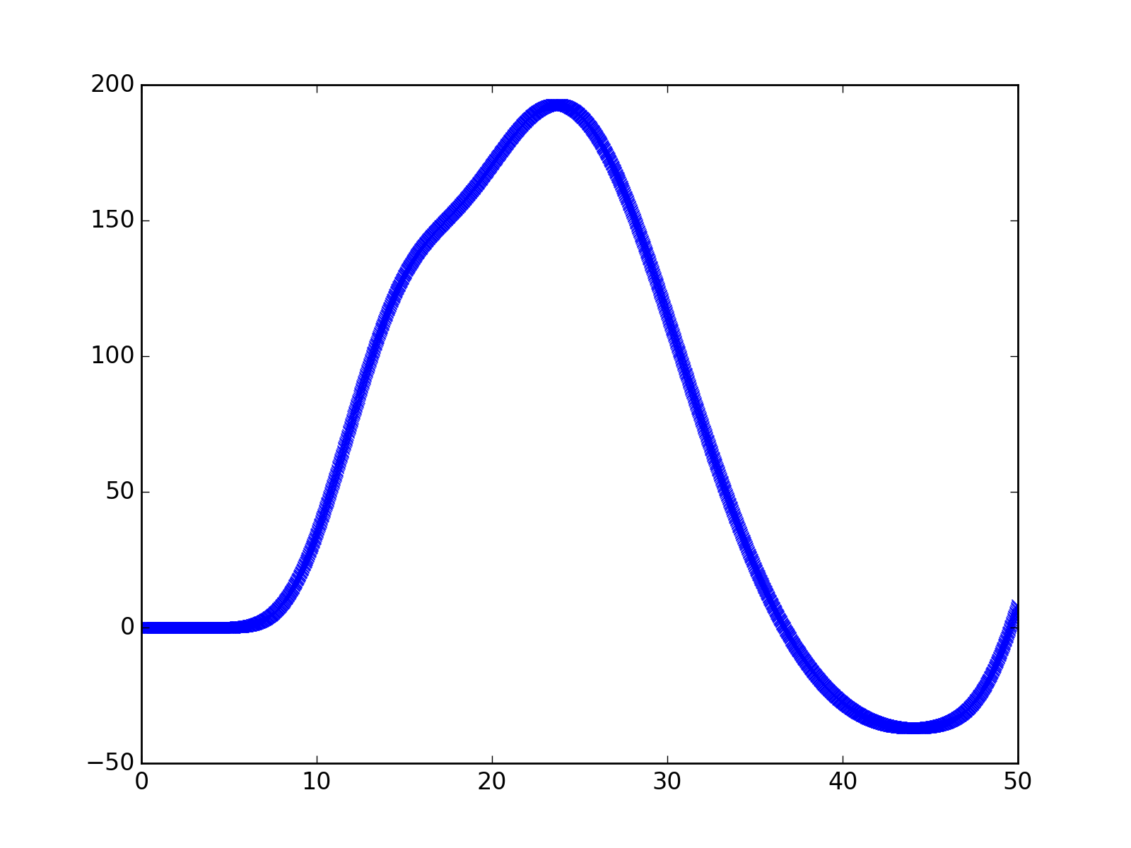
We can see that this is sampled at high resolution on the X axis by looking at the first 20 seconds-worth of data:

>>> plt.plot(high_res_times[:20 * tr_divs], high_res_hemo[:20 * tr_divs], 'x:')
[...]

(png, hires.png, pdf)

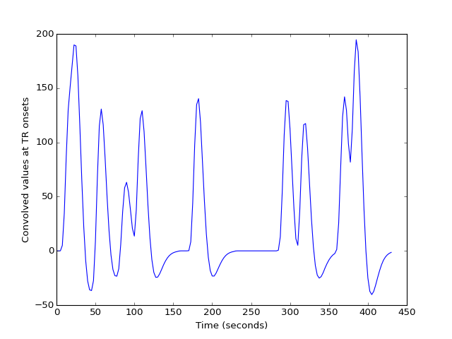
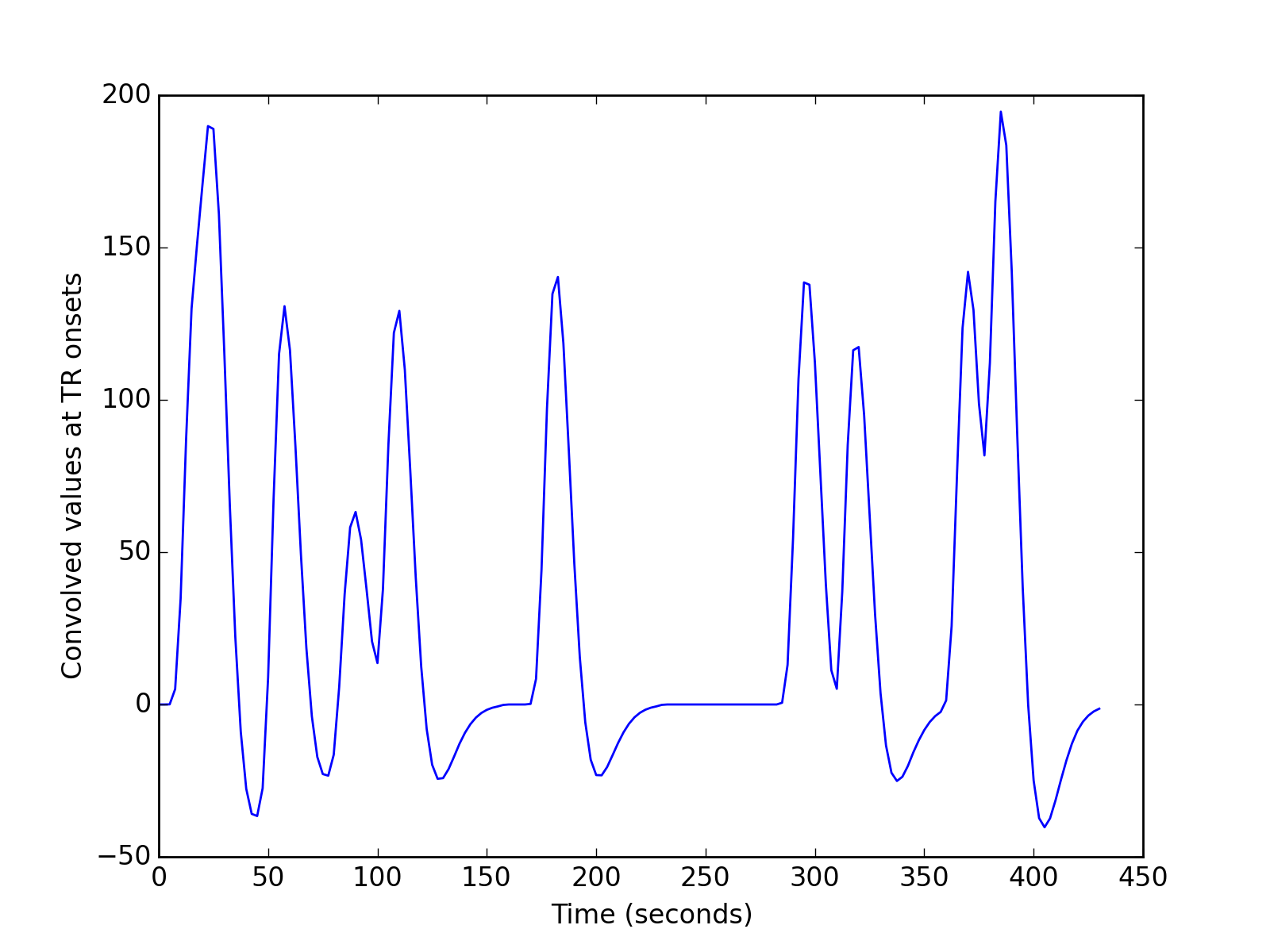
We can then subsample this high-resolution time course to get the values corresponding to the start of each original TR (volume):

>>> tr_indices = np.arange(n_trs)
>>> hr_tr_indices = np.round(tr_indices * tr_divs).astype(int)
>>> tr_hemo = high_res_hemo[hr_tr_indices]
>>> tr_times = tr_indices * TR  # times of TR onsets in seconds
>>> plt.plot(tr_times, tr_hemo)
[...]
>>> plt.xlabel('Time (seconds)')
<...>
>>> plt.ylabel('Convolved values at TR onsets')
<...>

(png, hires.png, pdf)

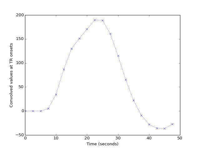
The first 20 seconds shows these values are sampled every TR rather than every 1/100th of a TR:

>>> plt.plot(tr_times[:20], tr_hemo[:20], 'x:')
[...]
>>> plt.xlabel('Time (seconds)')
<...>
>>> plt.ylabel('Convolved values at TR onsets')
<...>

(png, hires.png, pdf)