Working with four dimensional images, with some revision

Loading data with nibabel

First let’s load a three-dimensional file, like the one we were looking at last week.

import nibabel as nib

First we load the image, to give an “image” object:

img = nib.load('ds107_sub001_highres.nii')

You can explore the returned image object with img. followed by TAB in the IPython console.

Because images can have large arrays, nibabel does not load the image array when you load the image, in order to save time and memory. The best way to get the image array data is with the get_data() method.

data = img.get_data()
type(data)

This gives:

numpy.core.memmap.memmap

The memmap is a special type of array that saves memory, but otherwise behaves the same as any normal array.

The data is a three dimensional array. We can show slices from this data with matplotlib.

Four dimensional arrays - space + time

Images can also be four-dimensional. It’s easiest to think of four dimensional images as a stack of 3-dimensional images (volumes).

Here we load a four dimensional image. It is an functional MRI image, where the volumes are collected in sequence a few seconds apart.

img = nib.load('ds114_sub009_t2r1.nii')
data = img.get_data()

The image we have just loaded is a four-dimensional image, with a four-dimensional array:

data.shape

(64, 64, 30, 173)

The first three axes represent three dimensional space. The last axis represents time. Here the last (time) axis has length 173. This means that, for each of these 173 elements, there is one whole three dimensional image. We often call the three-dimensional images volumes. So we could say that this 4D image contains 173 volumes.

We have previously been taking slices over the third axis of a three-dimensional image. We can now take slices over the fourth axis of this four-dimensional image:

first_vol = data[:, :, :, 0]  # A slice over the final (time) axis

This slice selects the first three-dimensional volume (3D image) from the 4D array:

first_vol.shape

(64, 64, 30)

You can use the ellipsis ... when slicing an array. The ellipsis is a short cut for “everything on the previous axes”. For example, these two have exactly the same meaning:

first_vol = data[:, :, :, 0]
first_vol_again = data[..., 0]  # Using the ellipsis

first_vol is a 3D image just like the 3D images you have already seen:

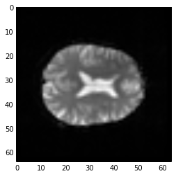
# A slice over the third dimension of a 3D image
plt.imshow(first_vol[:, :, 14], cmap='gray')

Numpy operations work on the whole array by default

Numpy operations like min, and max and std operate on the whole numpy array by default, ignoring any array shape. For example, here is the maximum value for the whole 4D array:

np.max(data)

6793

This is exactly the same as:

# maximum when flattening the array to 1 dimension
np.max(data.ravel())

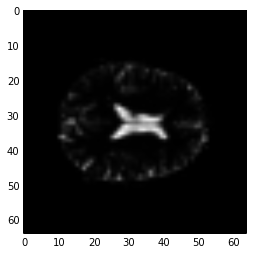
You can ask numpy to operate over particular axes instead of operating over the whole array. For example, this will generate a 3D image, where each array value is the variance over the 173 values at that 3D position (the variance across time):

# variance across the final (time) axis
var_vol = np.var(data, axis=3)
plt.imshow(var_vol[:, :, 14], cmap='gray')

Indexing with boolean arrays

We covered this briefly a few classes back.

Let’s say we have an array like this:

arr = np.array([[0, 1, 3, 0], [5, 2, 0, 1]])

We can get a True / False (boolean) array to tell us whether these values are above some threshold:

tf_array = arr > 2
tf_array

array([[False, False,  True, False],
       [ True, False, False, False]], dtype=bool)

You can flip the True / False values with ~ (bitwise not):

~tf_array

array([[ True,  True, False,  True],
       [False,  True,  True,  True]], dtype=bool)

We can use boolean arrays to index into the original array (or any array with a suitable shape). This will select only the elements where the boolean array is True. The returned array may well have selected only a few members from any particular row or column or (in general) higher axis, so the returned array is always one-dimensional to reflect the loss of shape:

selected_elements = arr[tf_array]
selected_elements

This gives:

array([3, 5])

The returned array is shape (2,) (one-dimensional).

We can use this to select values in our image as well. For example, if we wanted to select only values less than 10 in first_vol:

tf_lt_10 = first_vol < 10
vals_lt_10 = first_vol[tf_lt_10]
np.unique(vals_lt_10)

This gives:

array([0, 1, 2, 3, 4, 5, 6, 7, 8, 9], dtype=int16)