Using masks and modeling noise
Our usual setup:
>>> from __future__ import division
>>> import numpy as np
>>> import numpy.linalg as npl
>>> import matplotlib.pyplot as plt
Set defaults for plots:
>>> # set gray colormap and nearest neighbor interpolation by default
>>> plt.rcParams['image.cmap'] = 'gray'
>>> plt.rcParams['image.interpolation'] = 'nearest'
First we load our data, and slice off the first 4 volumes:
>>> import nibabel as nib
>>> img = nib.load('ds114_sub009_t2r1.nii')
>>> data = img.get_data()
>>> data = data[..., 4:]
>>> vol_shape = data.shape[:-1]
>>> n_trs = data.shape[-1]
>>> vol_shape, n_trs
((64, 64, 30), 169)
Next we take the mean volume (over time), and do a histogram of the values:
>>> mean_vol = np.mean(data, axis=-1)
>>> plt.hist(np.ravel(mean_vol), bins=100)
(...)
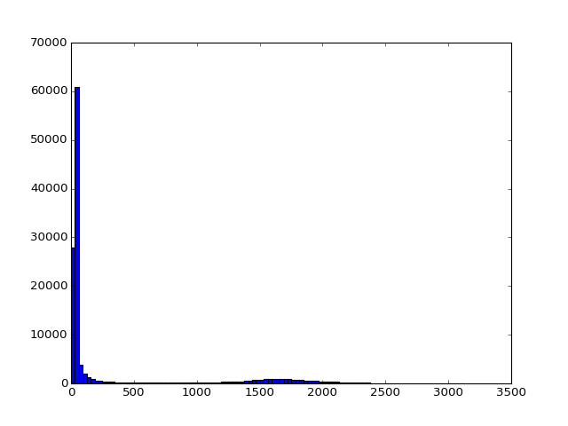
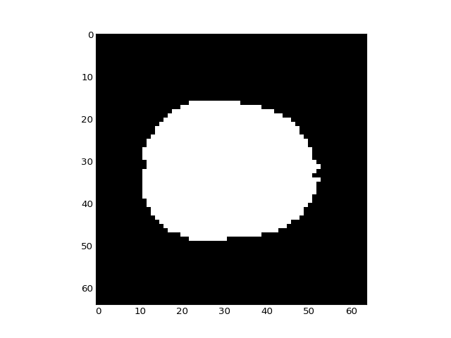
It looks like we can set a threshold to idenfity the voxels inside the brain. From this threshold we can get a 3D brain mask, that selects those voxels:
>>> in_brain_mask = mean_vol > 900
>>> in_brain_mask.shape
(64, 64, 30)
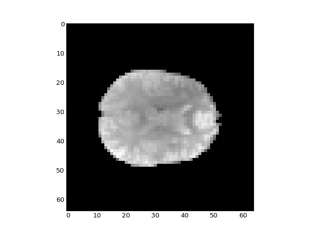
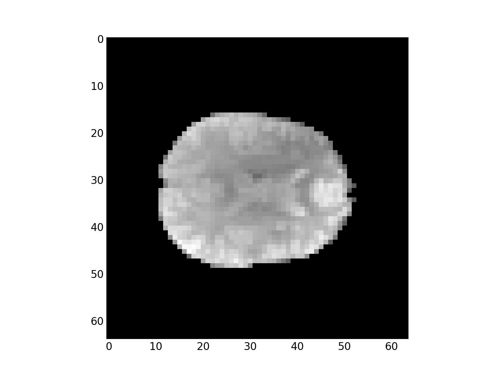
It looks this this has done a good job of selecting the voxels within the brain:
>>> plt.imshow(mean_vol[:, :, 14])
<...>

>>> plt.imshow(in_brain_mask[:, :, 14])
<...>

We can use this 3D mask to index into our 4D dataset. This selects all the voxel time-courses for voxels within the brain (as defined by the mask):
>>> in_brain_tcs = data[in_brain_mask, :]
>>> in_brain_tcs.shape
(21353, 169)
We can now run our model on just the time-courses for these voxels, rather than all voxels in the image.
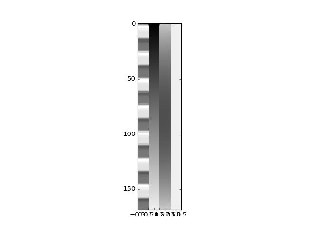
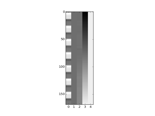
Let’s first try modeling our signals with an extra couple of drift terms. We will use a linear drift regressor, and a squared linear drift regressor:
>>> convolved = np.loadtxt('ds114_sub009_t2r1_conv.txt')[4:]
>>> X = np.ones((n_trs, 4))
>>> X[:, 0] = convolved
>>> linear_drift = np.linspace(-1, 1, n_trs)
>>> X[:, 1] = linear_drift
>>> quadratic_drift = linear_drift ** 2
>>> quadratic_drift -= np.mean(quadratic_drift)
>>> X[:, 2] = quadratic_drift
>>> plt.imshow(X, aspect=0.1)
<...>

We can fit this design to the data in the usual way:
>>> Y = in_brain_tcs.T
>>> B = npl.pinv(X).dot(Y)
>>> B.shape
(4, 21353)
There are four betas for each in-brain voxel. We can put these back into their correct voxel locations in the original 3D shape, by using the mask again:
>>> b_vols = np.zeros(vol_shape + (4,))
>>> b_vols[in_brain_mask, :] = B.T
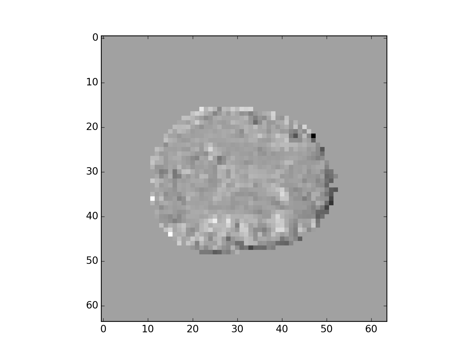
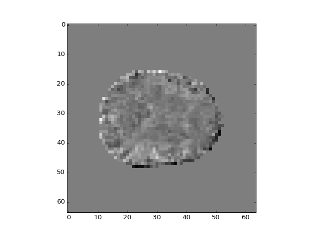
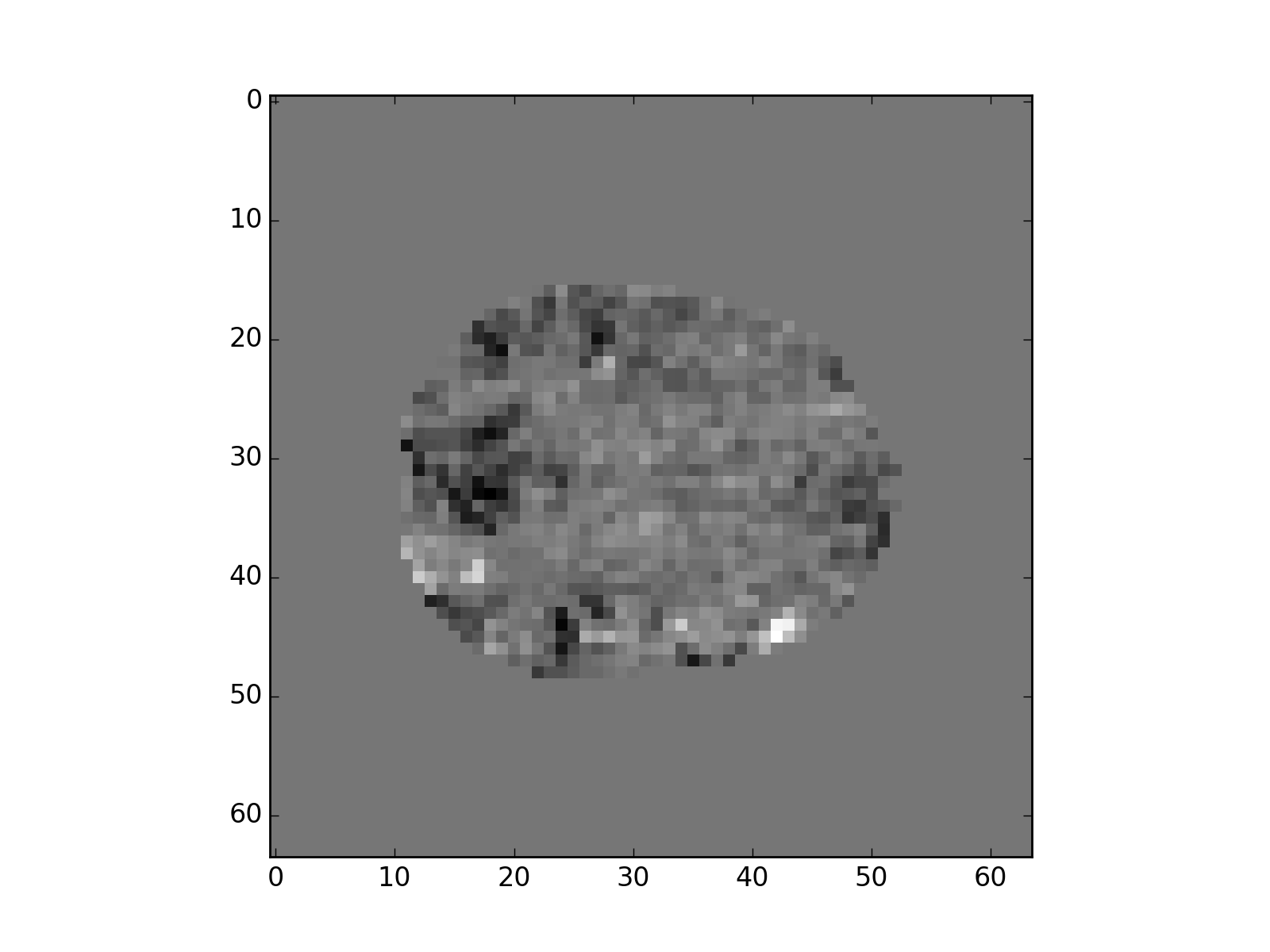
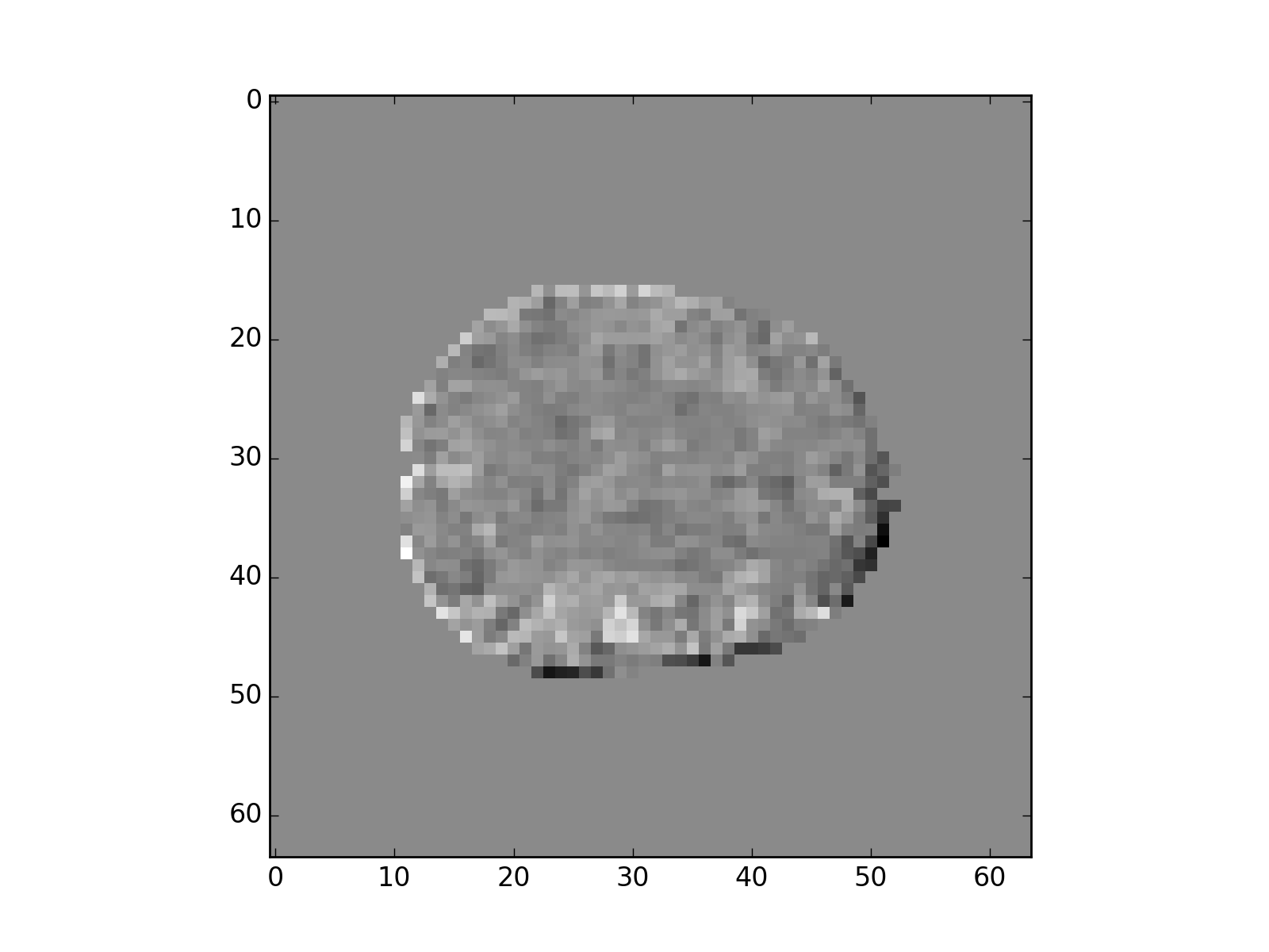
The different regressors pick up different patterns across the brain:
>>> plt.imshow(b_vols[:, :, 14, 0])
<...>
>>> plt.imshow(b_vols[:, :, 14, 1])
<...>

>>> plt.imshow(b_vols[:, :, 14, 2])
<...>

>>> plt.imshow(b_vols[:, :, 14, 3])
<...>
The drift terms model gradual drifts across the time-series, but are there other patterns of noise that we have not found yet? One way to look for such patterns is to use Principal Components Analysis:
>>> Y_demeaned = Y - np.mean(Y, axis=1).reshape([-1, 1])
>>> unscaled_cov = Y_demeaned.dot(Y_demeaned.T)
>>> U, S, V = npl.svd(unscaled_cov)
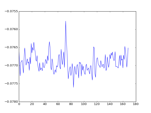
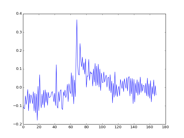
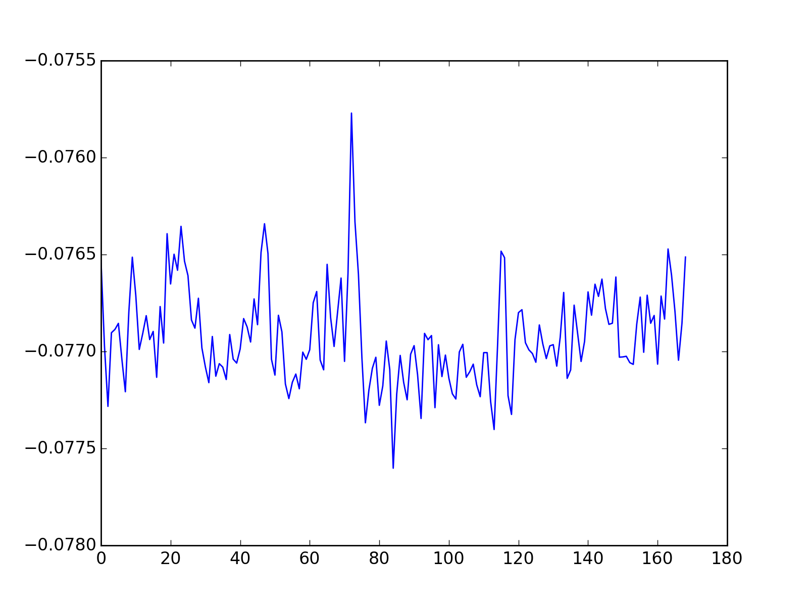
The component vectors (time-courses) are in the columns of the U matrix:
>>> plt.plot(U[:, 0])
[...]
We can get the projection of the data onto the new U basis with:
>>> projections = U.T.dot(Y_demeaned)
>>> projections.shape
(169, 21353)
Again, we can put these back into the correct 3D locations using the mask:
>>> projection_vols = np.zeros(data.shape)
>>> projection_vols[in_brain_mask, :] = projections.T
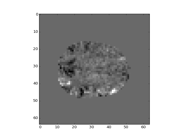
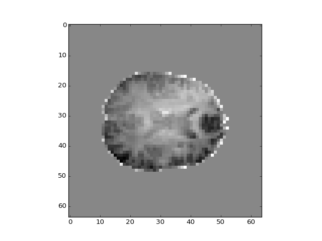
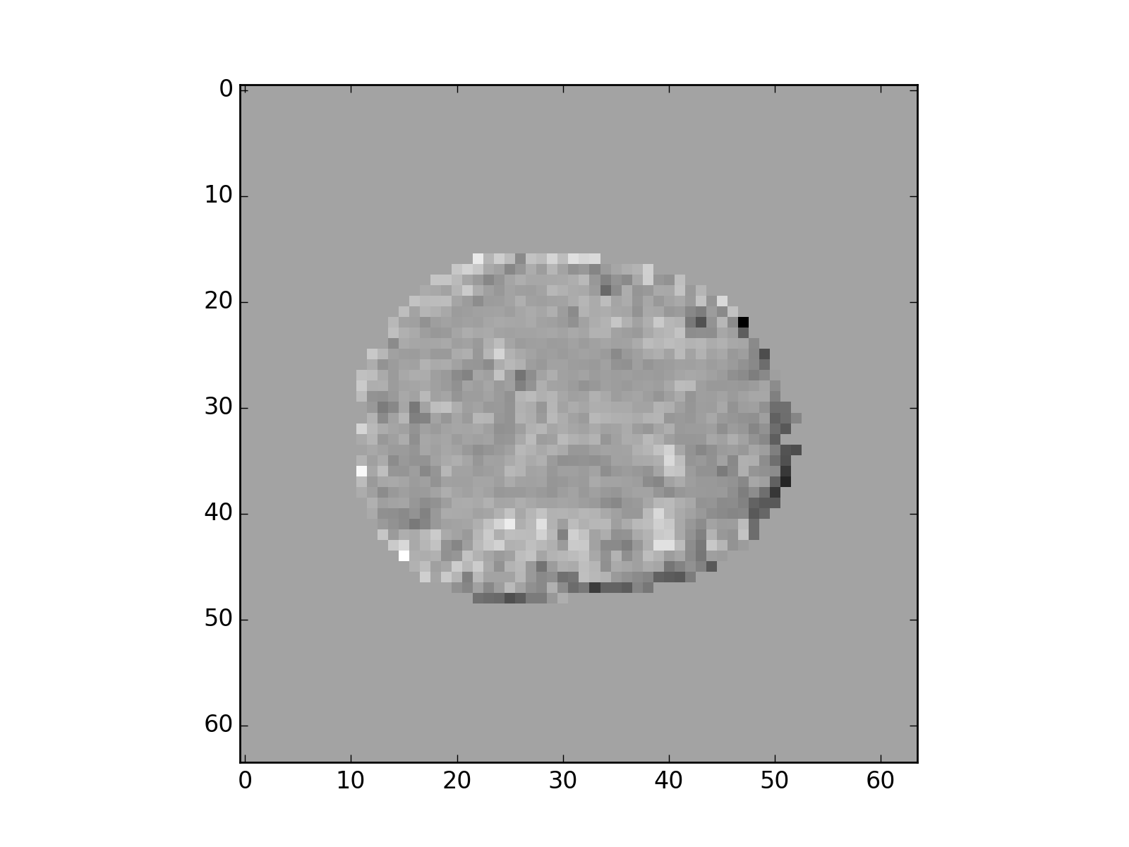
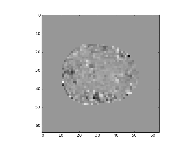
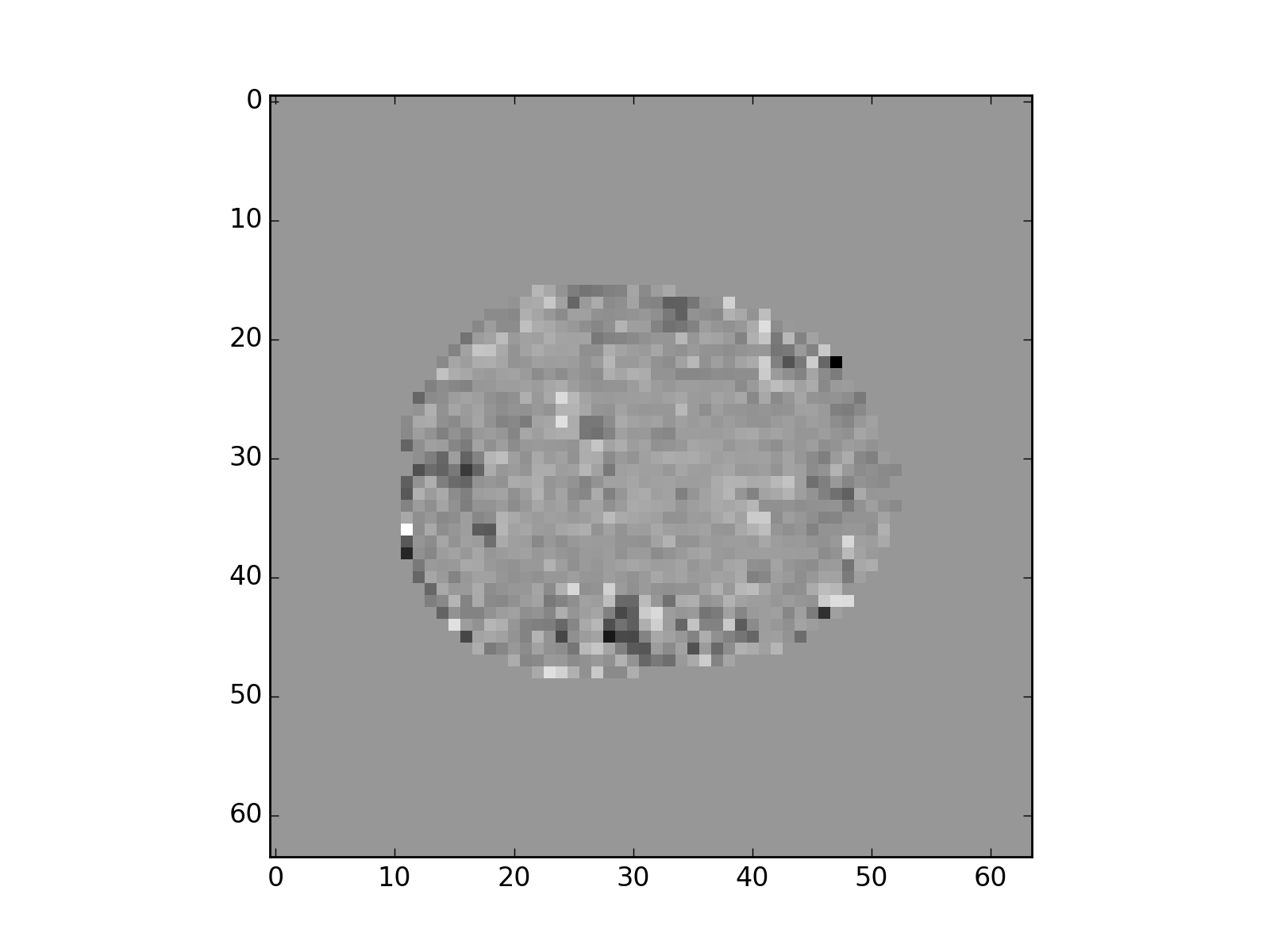
This first component doesn’t look like anything to do with the task:
>>> plt.imshow(projection_vols[:, :, 14, 0])
<...>
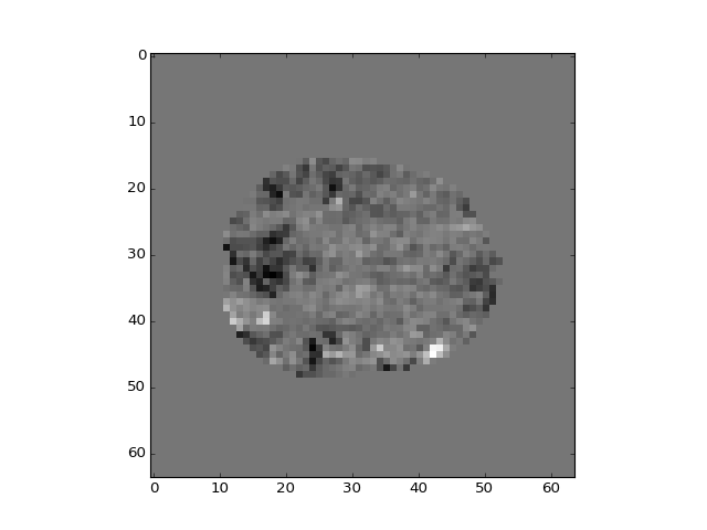
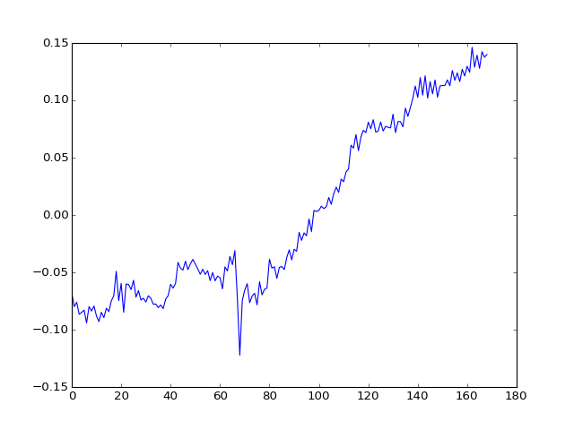
How about the second component?
>>> plt.plot(U[:, 1])
[...]

>>> plt.imshow(projection_vols[:, :, 14, 1])
<...>

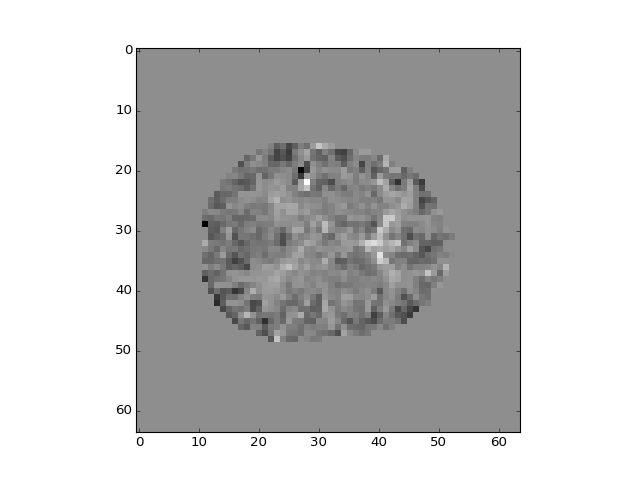
And the third?
>>> plt.plot(U[:, 2])
[...]
>>> plt.imshow(projection_vols[:, :, 14, 2])
<...>

At least the first two components look as if they are happening in many voxels at the same time, and they reflect brain anatomy rather than function. They may therefore reflect noise from the scanner or the subject. We can remove these components by regression:
>>> X_pca = np.ones((n_trs, 5))
>>> X_pca[:, 0] = convolved
>>> X_pca[:, 1:3] = U[:, :2]
>>> X_pca[:, 3] = linear_drift
>>> plt.imshow(X_pca, aspect=0.1)
<...>

>>> B_pca = npl.pinv(X_pca).dot(Y)
Again, we can put our fitted betas into their correct 3D location with the mask:
>>> b_pca_vols = np.zeros(vol_shape + (5,))
>>> b_pca_vols[in_brain_mask, :] = B_pca.T
>>> plt.imshow(b_pca_vols[:, :, 14, 0])
<...>
>>> plt.imshow(b_pca_vols[:, :, 14, 1])
<...>
>>> plt.imshow(b_pca_vols[:, :, 14, 2])
<...>

>>> plt.imshow(b_pca_vols[:, :, 14, 3])
<...>

