Testing a single voxel

A short ago (Modeling a single voxel), we were modeling a single voxel time course.

Let’s get that same voxel time course back again:

>>> import numpy as np
>>> import matplotlib.pyplot as plt
>>> import nibabel as nib

>>> img = nib.load('ds114_sub009_t2r1.nii')
>>> data = img.get_data()
>>> data = data[..., 4:]

The voxel coordinate (3D coordinate) that we were looking at before was at (42, 32, 19):

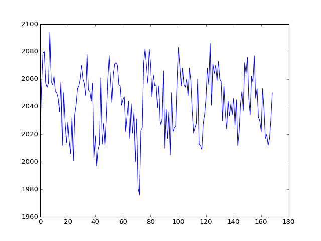
>>> voxel_time_course = data[42, 32, 19]
>>> plt.plot(voxel_time_course)
[...]

(png, hires.png, pdf)

We then compiled a design for this time-course and estimated it.

We used the convolved regressor from Convolving with the hemodyamic response function in a simple regression.

>>> convolved = np.loadtxt('ds114_sub009_t2r1_conv.txt')
>>> # Knock off first 4 elements to match data
>>> convolved = convolved[4:]
>>> N = len(convolved)
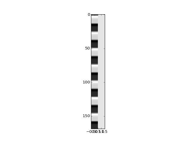
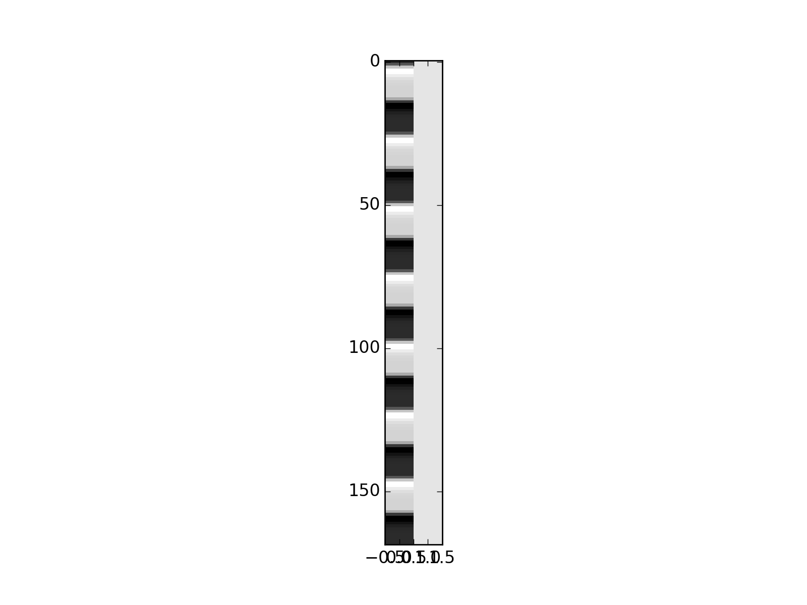
>>> X = np.ones((N, 2))
>>> X[:, 0] = convolved
>>> plt.imshow(X, interpolation='nearest', cmap='gray', aspect=0.1)
<...>

(png, hires.png, pdf)

\(\newcommand{\yvec}{\vec{y}}\) \(\newcommand{\xvec}{\vec{x}}\) \(\newcommand{\evec}{\vec{\varepsilon}}\) \(\newcommand{Xmat}{\boldsymbol X} \newcommand{\bvec}{\vec{\beta}}\) \(\newcommand{\bhat}{\hat{\bvec}} \newcommand{\yhat}{\hat{\yvec}}\)

As you will remember from Introduction to the general linear model, our model is:

\[\yvec = \Xmat \bvec + \evec\]

We can get our least squares parameter estimates for \(\bvec\) with:

\[\bhat = \Xmat^+y\]

where \(\Xmat^+\) is the pseudoinverse of \(\Xmat\). When \((\Xmat^T \Xmat)\) is invertible, the pseudoinverse is given by:

\[\Xmat^+ = (\Xmat^T \Xmat)^{-1} \Xmat^T\]

We find the \(\bhat\) for our data and design:

>>> import numpy.linalg as npl
>>> Xp = npl.pinv(X)
>>> beta_hat = Xp.dot(voxel_time_course)
>>> beta_hat
array([   31.185514,  2029.367685])

Our plan now is to do an hypothesis test on our \(\bhat\) values.

The \(\bhat\) values are sample estimates of the unobservable true \(\bvec\) parameters.

Because the \(\bhat\) values are sample estimates, the values we have depend on the particular sample we have, and the particular instantiation of the random noise (residuals). If we were to take another set of data from the same voxel during the same task, we would get another estimate, because there would be different instantiation of the random noise. It’s possible to show that the variance / covariance of the \(\hat\beta\) estimates is:

\[\text{Cov}(\hat\beta) = \sigma^2 \left(X^T X\right)^{-1}.\]

where \(\sigma^2\) is the true unknown variance of the errors. See wikipedia proof, and stackoverflow proof.

We can use an estimate \(s^2\) of \(\sigma^2\) to give us estimated standard errors of the variance covariance:

>>> y = voxel_time_course
>>> y_hat = X.dot(beta_hat)
>>> residuals = y - y_hat
>>> # Residual sum of squares
>>> RSS = np.sum(residuals ** 2)
>>> # Degrees of freedom
>>> df = X.shape[0] - npl.matrix_rank(X)
>>> # Mean residual sum of squares
>>> MRSS = RSS / df
>>> # This is our s^2
>>> s2 = MRSS
>>> print(s2)
247.937561534
>>> print(np.sqrt(s2))
15.7460332

We now have an standard estimate of the variance / covariance of the \(\bhat\):

>>> v_cov = s2 * npl.inv(X.T.dot(X))

In particular, I can now divide my estimate for the first parameter, by the standard error of that estimate:

>>> numerator = beta_hat[0]
>>> denominator = np.sqrt(v_cov[0, 0])
>>> t_stat = numerator / denominator
>>> print(t_stat)
12.8267805905

I can look up the probability of this t statistic using scipy.stats:

>>> from scipy.stats import t as t_dist
>>> # Get p value for t value using cumulative density dunction
>>> # (CDF) of t distribution
>>> ltp = t_dist.cdf(t_stat, df) # lower tail p
>>> p = 1 - ltp # upper tail p
>>> p
0.0

Finally let’s save the voxel time course for us to use in R:

>>> np.savetxt('voxel_time_course.txt', voxel_time_course)